N or Space for next slide, P for previous slide, F for full screen, M for menu
Lec 9: NAND shift
Boaz Barak (instructor), Salil Vadhan (co-instructor), Juan Perdomo (Head TF).
Team: Aditya Mahadevan, Brian Sapozhnikov (surveys), Chan Kang (extension), Gabe Abrams (Ed Tech), Gabe Montague (NAND web), Jessica Zhu (proof workshops), John Shen, Juan Esteller (NAND implementation), Karl Otness, Katherine Binney, Lisa Lu, Mark Goldstein (clicker expert), Stefan Spataru, Susan Xu, Tara Sowrirajan, Thomas Orton (Advanced Section)
Slides will be posted online.

Laptops/phones only on last 3 rows please.
Thursday: NAND++ and Turing machines
- Model to compute an infinite function \(F:\{0,1\}^* \rightarrow \{0,1\}^*\).
Two components:
Local storage - states (Turing machines) or scalar variables and current line (NAND++).
Unbounded size memory - tape (Turing machines) or array variables (NAND++)
Sequential access - head location (Turing machine) or index variable
imoves one step at a time.
Random Access Memory (RAM): Can access arbitrary memory location.
In C:
foo = *barorfoo = Array[bar]In Python:
foo = Array[bar]In NAND<< :
foo = Array[bar]
NAND<<
Convention: foo is scalar, Bar is array. Bar[foo] is foo-th location at Bar
Today: NAND<<, lambda calculus, finite automata
NAND++: Minimal extension to NAND to allow infinite functions. One global loop
Memory access both oblivious and sequential
NAND<<: Standard RAM model. “Random access” to memory (query access \(i \mapsto A[i]\)) Standard arithmetic operations on integers (addition, subtraction, multiplication, division, mod, comparison), use integers as indices to arrays.
One “caveat”: In \(T\) time can only handle integers in \(\{0,\ldots,T-1\}\).
Captures essentially all features of modern programming languages.
Question
Let \(D\) := NAND++ computable functions and \(D'\) := NAND<< computable functions.
Which of the following holds:
a. There is a one-to-one map from \(D\) to \(D'\)
b. There is a one-to-one map from \(D'\) to \(D\)
c. There is an onto map from \(D\) to \(D'\).
d. There is an onto map from \(D'\) to \(D\).
e. All of the above.
Today’s Theorems
Thm 6: \(D=D'\): \(F\) is computable by a NAND++ program if and only if \(F\) is computable by a NAND<< program.
Thm 7: \(EVAL\) is computable by NAND++, where \(EVAL(P,x)=P(x)\) for every \(x\) on which \(P\) halts.
Outline proof of Thms
Discuss why it’s important
High level vs low level description
High level vs low level description
Three levels of descriptions of NAND++ programs.
- Low level: Precise code or tuple representation.
- Implementation level: (“Pseudocode”) Outline NAND++ program structure in English. Can also appeal to syntactic sugar.
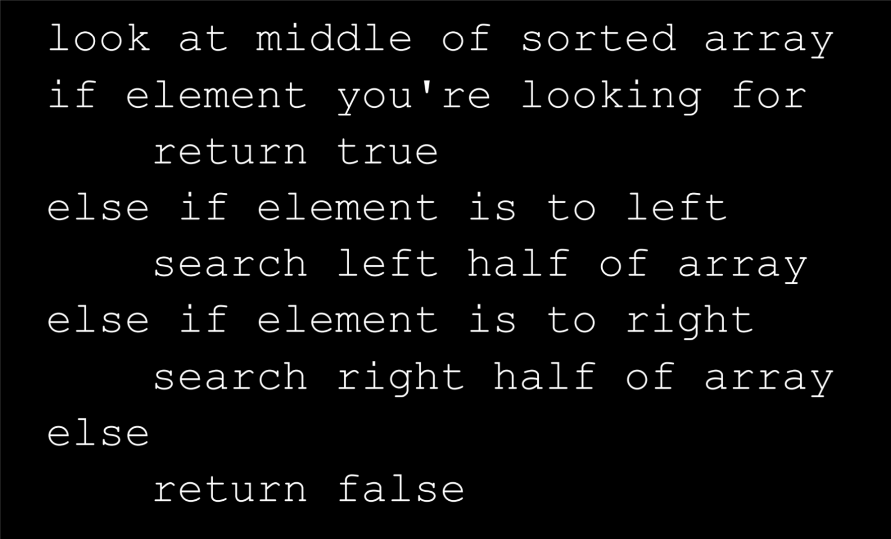
- High level: Describe algorithm at high level, just like CS 50 or CS 124. Trust it’s always possible to convert to NAND++ if needed.
This course: We’ll say what we level is expected.
Three levels of description of objects
- Low level: Precise encoding as bit string (e.g., \(G=(V,E)\) is encoded as \([ [i_0,j_0],\ldots, [i_{m-1},j_{m-1}]]\) where \(E=\{(i_k,j_k)\}_{k\in [m]}\) and we encode \(\{"[",","]",0,1\}\) to \(\{0,1\}^3\) by the map \("[" \mapsto 000\), \("," \mapsto 001\), \("]" \mapsto 010\), \(0 \mapsto 011\), \(1 \mapsto 100\))
- Implementation level: Describe map to strings in English. (e.g., \(G\) is mapped to string by encoding as adjacency list and encoding the list as string)
- High level: Assume some canonical representation is implied. (e.g., program \(P\) takes a graph \(G\) as input.)
This course: We’ll say what we level is expected.
The YCHYCAEIT paradigm
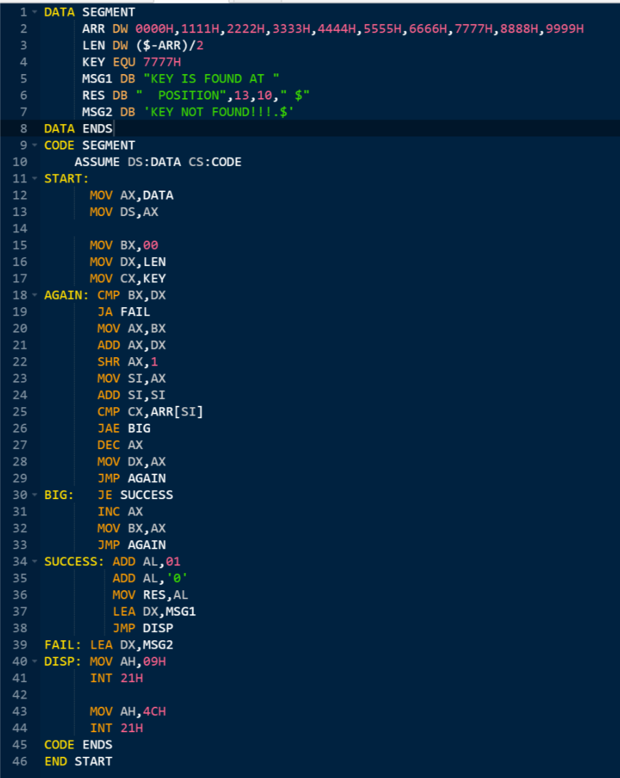
- To prove function is computable, use NAND<< or even higher level descriptions. (“pseudocode” / “algorithms”)
- To prove function is uncomputable, use NAND++ or even more restricted versions (“simple NAND++ programs”)
If you can think it
..then you can code it
..then you can NAND<< it
..then you can NAND++ it.
Today’s Theorems
Thm 6: \(D=D'\): \(F\) is computable by a NAND++ program if and only if \(F\) is computable by a NAND<< program.
Thm 7: \(EVAL\) is computable by NAND++, where \(EVAL(P,x)=P(x)\) for every \(x\) on which \(P\) halts.
Universal NAND++ program
Thm: Let \(EVAL(P,x) = P(x)\) for every NAND++ program \(P\in \{0,1\}^*\) and \(x\in \{0,1\}^*\) s.t. \(P\) halts on \(x\). Then \(EVAL\) is NAND++-computable.
Proof: Can give pseudocode for \(EVAL\) \(\Rightarrow\) \(EVAL\) is Python computable \(\Rightarrow\) \(EVAL\) is NAND<< computable \(\Rightarrow\) \(EVAL\) is NAND++ computable
We’ll do Steps 1 (pseudocode) and 2 (Python)
Computing EVAL
Input: 1) Description of NAND++ program: list \(L\) of \(6\)-tuples: \((a,j,b,k,c,\ell)\) corresponds to \(a_j := b_k NAND c_\ell\).
2) \(x \in \{0,1\}^n\)
Operation: Let \(s=|L|\). Have \(3s \times T\) array \(A\). (Initially \(T=n\), expand as needed)
1. Set \(A[0][i] = x_i\) and \(A[2][i]=1\) for \(i\in [n]\). (x,validx)
2. Set \(i=0\),\(idxinc=1\),\(r=0\).
- For \((a,j,b,k,c,\ell) \in L\):
- Change indices to \(i\) if they equal \(s\).
- Set \(A[a][j] = 1 - A[b][k]*A[c][\ell]\)
4. If \(idxinc=1\) then set \(i=i+1\) else set \(i=i-1\).
5. If \(i=r+1\) then set \(r=r+1\), \(idxinc=0\). If \(i=0\) then set \(idxinc=1\)
6. If \(A[3][0]=1\) then goto 3.
Python: in notebook
From NAND++ to NAND<< in 7 easy steps
Thm 6: \(D=D'\): \(F\) is computable by a NAND++ program if and only if \(F\) is computable by a NAND<< program.
1: Controlling the index and inner loops. \(i++\) , \(--\), \(while\)
2: Operations on integers. \(ADD\), \(MULT\), ..
3: Set index to desired location.
4: Maintaining a program counter and index.
5: Two dim bit arrays.
6: One dim integer arrays
7: Simulating NAND<<
Peeling NAND<<
- Simulate integer arrays by one dim arrays__
- Simulate \(i:=foo\) with \(i++,i--\)
- Simulate \(i++,i--\) with breadcrumbs
Breadcrumbs
- \(atstart_0=1\), \(atstart_i=0\) for \(i \neq 0\).
- \(breadcrumbs_i=1\) if \(i\) was seen before
Accounting
- Simulating \(i++,i--\): increases \(T\) steps to \(O(T^2)\).
- Simulating \(i := foo\): another \(T\) to \(O(T^2)\) increase.
- Integer addition, product, multiplication: \(poly(\log T) = o(T)\).
Total overhead: \(O(T^5)\).
Universal NAND++ program
Thm: Let \(EVAL(P,x) = P(x)\) for every NAND++ program \(P\in \{0,1\}^*\) and \(x\in \{0,1\}^*\) s.t. \(P\) halts on \(x\). Then \(EVAL\) is NAND++-computable.
Proof: \(EVAL\) is Python computable \(\Rightarrow\) \(EVAL\) is NAND<< computable \(\Rightarrow\) \(EVAL\) is NAND++ computable
\(\lambda\) calculus
If \(f = \lambda x.e\) then \(f y\) is \(e[x \rightarrow y]\).
Currying \(\lambda x,y. exp = \lambda x.(\lambda y. exp)\)
Precedence rule: \(f x y = (f x) y\).
Question: Suppose that \(F = \lambda f. (\lambda x. (f x)f)\), \(1 = \lambda x.(\lambda y.x)\) and \(0=\lambda x.(\lambda y.y)\). What is \(F \; 1\; 0\)?
a. \(1\)
b. \(0\)
c. \(\lambda x.1\)
d. \(\lambda x.0\)
\(\lambda\)-computability
Informal: \(F\) is \(\lambda\)-computable if equal to \(\lambda\) expression.
Recall: \(NIL\) - empty list, \(PAIR\) - create pair. List \((a,b,c) = PAIR \; a \; (PAIR \; b \; (PAIR\; c \; NIL))\)
Formal: \(F:\{0,1\}^* \rightarrow \{0,1\}\) is \(\lambda\)-computable if exists \(\lambda\)-expression \(e\) such that for every \(x\in \{0,1\}^n\), \(F(x_0,\ldots,x_{n-1})\) equals
Thm: \(F\) is \(\lambda\)-computable iff \(F\) is NAND++ computable.
Proof: \(\Rightarrow\): repeat “search and replace” to evaluate \(\lambda\) expressions.
\(\Leftarrow\): crucial insight is \(NEXT_P\) is computable by “search and replace”
Preliminaries
- Set \(0 = \lambda x,y.y\) and \(1= \lambda x,y.x\). Then \(IF \; cond \; a \; b = cond \; a \; b\).
- Set \(PAIR = \lambda x,y. (\lambda f. f x y)\), \(HEAD = 1\), \(TAIL = 0\).
- \(NIL = \lambda f.1\), \(ISNIL\; P = P (\lambda x,y.0)\).
To define \(MAP\), \(FILTER\), \(REDUCE\) we need recursion
Y combinator
Turing Eret @turingmachine
Hat-tip: Matt Might (see also Y combinator in Javascript)
Y combinator
Example:
Question: Why is this a recursive definition for \(PAR\; L\)?
Non recursive function:
Lemma: \(PAR = APAR \; APAR\) satisfies equation \(\color{red}{(*)}\)
Proof: Plug \(f=APAR\) in \(\color{green}{(**)}\).
Cor: \(PAR \; L\) is the parity of \(L\) for every list \(L\).
Y combinator
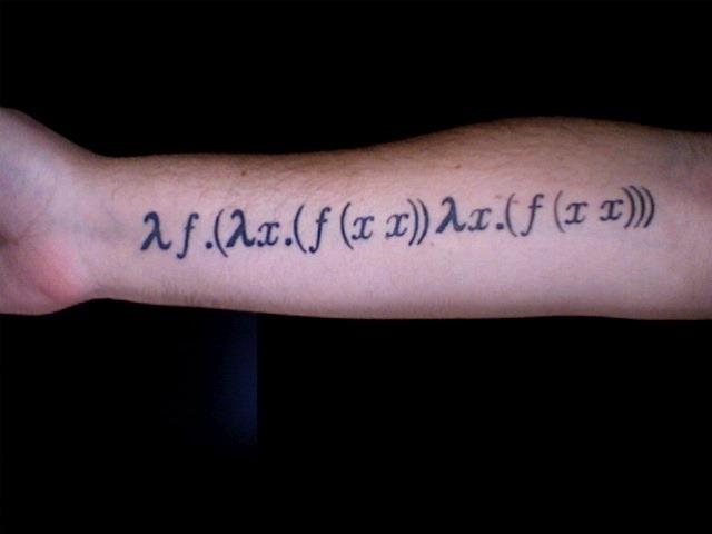
Thm: Let \(Y = \lambda f. (\lambda x. f (x\; x)) (\lambda y. f (y\; y))\). Then for every \(F\), \(f=YF\) solves the recursive/fixed-point equation \(f=F\; f\).
Pf: Write
\(Y\; F = \color{green}{(\lambda x. F (x\; x))} \color{red}{(\lambda y. F (y\; y))}\) =\(\color{green}{F (x\; x)}[x \rightarrow \color{red}{\lambda y.F(y \; y)}]\)
=\(\color{green}{F(}\color{red}{(\lambda y.F(y \; y))} \; \color{red}{(\lambda y.F(y \; y))} \color{green}{)}\)
=\(F(Y F)\)
Using this can define \(FILTER\),\(MAP\),\(REDUCE\), etc..
Simulate NAND++ with \(\lambda\)
Simulate \(NEXT_P\)
Recursively repeat until halt
- Configuration: list of blocks
Crucial observations:
- \(\lambda\) can do AND/OR/NOT \(\Rightarrow\) any finite function
- Next configuration is obtained by finite function applied to finitely many blocks. \(\Rightarrow\) \(FILTER\) to find active block and then constantly many applications of \(MAP\)/\(REDUCE\)
Church-Turing Thesis
“Computable” \(\approx\) TM-computable
= \(\lambda\)-computable
= NAND++ computable
= NAND<< computable
= Python-computable
\(\approx\) “Human computable”
\(\approx\) “Alien computable”
= ….
Highlighted Theorems on NAND
Thm 1: NAND programs \(\equiv\) NAND circuits \(\equiv\) AND/OR/NOT circuits \(\equiv\) \(\mathscr{U}\)-circuits, for any universal \(\mathscr{U}\).
Thm 2: Every function \(F:\{0,1\}^n \rightarrow \{0,1\}\) has a NAND program of \(O(2^n)\) lines. (in fact \(O(2^n/m)\)) (many functions require much fewer lines)
Thm 3: Some (in fact most) functions \(F:\{0,1\}^n \rightarrow \{0,1\}\) require NAND programs of \(\Omega(2^n/n)\) lines.
Thm 4: \(EVAL_{s,n,m} \in Size(poly(s))\).
Thm 5: (informal) NAND \(\cong\) NAND + sugar “If you can Python it, you can NAND it”